Time Series Forecasting: A Practical Guide to Exploratory Data Analysis

Introduction
Time series analysis certainly represents one of the most widespread topics in the field of Data Science and machine learning: whether predicting financial events, energy consumption, product sales or stock market trends, this field has always been of great interest to businesses.
Obviously, the great increase in data availability, combined with the constant progress in machine learning models, has made this topic even more interesting today. Alongside traditional forecasting methods derived from statistics (e.g. regressive models, ARIMA models, exponential smoothing), techniques relating to machine learning (e.g. tree-based models) and deep learning (e.g. LSTM Networks, CNNs, Transformer-based Models) have emerged for some time now.
Despite the huge differences between these techniques, there is a preliminary step that must be done, no matter what the model is: Exploratory Data Analysis.
In statistics, Exploratory Data Analysis (EDA) is a discipline consisting in analyzing and visualizing data in order to summarize their main characteristics and gain relevant information from them. This is of considerable importance in the data science field because it allows to lay the foundations to another important step: feature engineering. That is, the practice that consists on creating, transforming and extracting features from the dataset so that the model can work to the best of its possibilities.
The objective of this article is therefore to define a clear exploratory data analysis template, focused on time series, which can summarize and highlight the most important characteristics of the dataset. To do this, we will use some common Python libraries such as Pandas, Seaborn and Statsmodel.
Data
Let's first define the dataset: for the purposes of this article, we will take Kaggle's Hourly Energy Consumption data. This dataset relates to PJM Hourly Energy Consumption data, a regional transmission organization in the United States, that serves electricity to Delaware, Illinois, Indiana, Kentucky, Maryland, Michigan, New Jersey, North Carolina, Ohio, Pennsylvania, Tennessee, Virginia, West Virginia, and the District of Columbia.
The hourly power consumption data comes from PJM's website and are in megawatts (MW).
Exploratory Data Analysis
Let's now define which are the most significant analyses to be performed when dealing with time series.
For sure, one of the most important thing is to plot the data: graphs can highlight many features, such as patterns, unusual observations, changes over time, and relationships between variables. As already said, the insight that emerge from these plots must then be taken into consideration, as much as possible, into the forecasting model. Moreover, some mathematical tools such as descriptive statistics and time series decomposition, will also be very useful.
Said that, the EDA I'm proposing in this article consists on six steps: Descriptive Statistics, Time Plot, Seasonal Plots, Box Plots, Time Series Decomposition, Lag Analysis.
1. Descriptive Statistics
Descriptive statistic is a summary statistic that quantitatively describes or summarizes features from a collection of structured data.
Some metrics that are commonly used to describe a dataset are: measures of central tendency (e.g. mean, median), measures of dispersion (e.g. range, standard deviation), and measure of position (e.g. percentiles, quartile). All of them can be summarized by the so called five number summary, which include: minimum, first quartile (Q1), median or second quartile (Q2), third quartile (Q3) and maximum of a distribution.
In Python, these information can be easily retrieved using the well know describe method from Pandas:
import pandas as pd

# Loading and preprocessing steps
df = pd.read_csv('../input/hourly-energy-consumption/PJME_hourly.csv')
df = df.set_index('Datetime')
df.index = pd.to_datetime(df.index)

df.describe()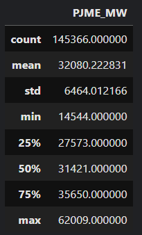
2. Time plot
The obvious graph to start with is the time plot. That is, the observations are plotted against the time they were observed, with consecutive observations joined by lines.
In Python , we can use Pandas and Matplotlib:
import matplotlib.pyplot as plt

# Set pyplot style
plt.style.use("seaborn")

# Plot
df['PJME_MW'].plot(title='PJME - Time Plot', figsize=(10,6))
plt.ylabel('Consumption [MW]')
plt.xlabel('Date')
This plot already provides several information:
- As we could expect, the pattern shows yearly seasonality.
- Focusing on a single year, it seems that more pattern emerges. Likely, the consumptions will have a peak in winter and one another in summer, due to the greater electricity consumption.
- The series does not exhibit a clear increasing/decreasing trend over the years, the average consumptions remains stationary.
- There is an anomalous value around 2023, probably it should be imputed when implementing the model.
3. Seasonal Plots
A seasonal plot is fundamentally a time plot where data are plotted against the individual "seasons" of the series they belong.
Regarding energy consumption, we usually have hourly data available, so there could be several seasonality: yearly, weekly, daily. Before going deep into these plots, let's first set up some variables in our Pandas dataframe:
# Defining required fields
df['year'] = [x for x in df.index.year]
df['month'] = [x for x in df.index.month]
df = df.reset_index()
df['week'] = df['Datetime'].apply(lambda x:x.week)
df = df.set_index('Datetime')
df['hour'] = [x for x in df.index.hour]
df['day'] = [x for x in df.index.day_of_week]
df['day_str'] = [x.strftime('%a') for x in df.index]
df['year_month'] = [str(x.year) + '_' + str(x.month) for x in df.index]
3.1 Seasonal plot – Yearly consumption
A very interesting plot is the one referring to the energy consumption grouped by year over months, this highlights yearly seasonality and can inform us about ascending/descending trends over the years.
Here is the Python code:
import numpy as np

# Defining colors palette
np.random.seed(42)
df_plot = df[['month', 'year', 'PJME_MW']].dropna().groupby(['month', 'year']).mean()[['PJME_MW']].reset_index()
years = df_plot['year'].unique()
colors = np.random.choice(list(mpl.colors.XKCD_COLORS.keys()), len(years), replace=False)

# Plot
plt.figure(figsize=(16,12))
for i, y in enumerate(years):
    if i > 0:
        plt.plot('month', 'PJME_MW', data=df_plot[df_plot['year'] == y], color=colors[i], label=y)
        if y == 2018:
            plt.text(df_plot.loc[df_plot.year==y, :].shape[0]+0.3, df_plot.loc[df_plot.year==y, 'PJME_MW'][-1:].values[0], y, fontsize=12, color=colors[i])
        else:
            plt.text(df_plot.loc[df_plot.year==y, :].shape[0]+0.1, df_plot.loc[df_plot.year==y, 'PJME_MW'][-1:].values[0], y, fontsize=12, color=colors[i])

# Setting labels
plt.gca().set(ylabel= 'PJME_MW', xlabel = 'Month')
plt.yticks(fontsize=12, alpha=.7)
plt.title("Seasonal Plot - Monthly Consumption", fontsize=20)
plt.ylabel('Consumption [MW]')
plt.xlabel('Month')
plt.show()
This plot shows every year has actually a very predefined pattern: the consumption increases significantly during winter and has a peak in summer (due to heating/cooling systems), while has a minima in spring and in autumn when no heating or cooling is usually required.
Furthermore, this plot tells us that's not a clear increasing/decreasing pattern in the overall consumptions across years.
3.2 Seasonal plot – Weekly consumption
Another useful plot is the weekly plot, it depicts the consumptions during the week over months and can also suggest if and how weekly consumptions are changing over a single year.
Let's see how to figure it out with Python:
# Defining colors palette
np.random.seed(42)
df_plot = df[['month', 'day_str', 'PJME_MW', 'day']].dropna().groupby(['day_str', 'month', 'day']).mean()[['PJME_MW']].reset_index()
df_plot = df_plot.sort_values(by='day', ascending=True)

months = df_plot['month'].unique()
colors = np.random.choice(list(mpl.colors.XKCD_COLORS.keys()), len(months), replace=False)

# Plot
plt.figure(figsize=(16,12))
for i, y in enumerate(months):
    if i > 0:
        plt.plot('day_str', 'PJME_MW', data=df_plot[df_plot['month'] == y], color=colors[i], label=y)
        if y == 2018:
            plt.text(df_plot.loc[df_plot.month==y, :].shape[0]-.9, df_plot.loc[df_plot.month==y, 'PJME_MW'][-1:].values[0], y, fontsize=12, color=colors[i])
        else:
            plt.text(df_plot.loc[df_plot.month==y, :].shape[0]-.9, df_plot.loc[df_plot.month==y, 'PJME_MW'][-1:].values[0], y, fontsize=12, color=colors[i])

# Setting Labels
plt.gca().set(ylabel= 'PJME_MW', xlabel = 'Month')
plt.yticks(fontsize=12, alpha=.7)
plt.title("Seasonal Plot - Weekly Consumption", fontsize=20)
plt.ylabel('Consumption [MW]')
plt.xlabel('Month')
plt.show()
3.3 Seasonal plot – Daily consumption
Finally, the last seasonal plot I want to show is the daily consumption plot. As you can guess, it represents how consumption change over the day. In this case, data are first grouped by day of week and then aggregated taking the mean.
Here's the code:
import seaborn as sns

# Defining the dataframe
df_plot = df[['hour', 'day_str', 'PJME_MW']].dropna().groupby(['hour', 'day_str']).mean()[['PJME_MW']].reset_index()

# Plot using Seaborn
plt.figure(figsize=(10,8))
sns.lineplot(data = df_plot, x='hour', y='PJME_MW', hue='day_str', legend=True)
plt.locator_params(axis='x', nbins=24)
plt.title("Seasonal Plot - Daily Consumption", fontsize=20)
plt.ylabel('Consumption [MW]')
plt.xlabel('Hour')
plt.legend()
Often, this plot show a very typical pattern, someone calls it "M profile" since consumptions seems to depict an "M" during the day. Sometimes this pattern is clear, others not (like in this case).
However, this plots usually shows a relative peak in the middle of the day (from 10 am to 2 pm), then a relative minima (from 2 pm to 6 pm) and another peak (from 6 pm to 8 pm). Finally, it also shows the difference in consumptions from weekends and other days.
3.4 Seasonal plot – Feature Engineering
Let's now see how to use this information for feature engineering. Let's suppose we are using some ML model that requires good quality features (e.g. ARIMA models or tree-based models).
These are the main evidences coming from seasonal plots:
- Yearly consumptions do not change a lot over years: this suggests the possibility to use, when available, yearly seasonality features coming from lag or exogenous variables.
- Weekly consumptions follow the same pattern across months: this suggests to use weekly features coming from lag or exogenous variables.
- Daily consumption differs from normal days and weekends: this suggest to use categorical features able to identify when a day is a normal day and when it is not.
4. Box Plots
Boxplot are a useful way to identify how data are distributed. Briefly, boxplots depict percentiles, which represent 1st (Q1), 2nd (Q2/median) and 3rd (Q3) quartile of a distribution and whiskers, which represent the range of the data. Every value beyond the whiskers can be thought as an outlier, more in depth, whiskers are often computed as:

4.1 Box Plots – Total consumption
Let's first compute the box plot regarding the total consumption, this can be easily done with Seaborn:
plt.figure(figsize=(8,5))
sns.boxplot(data=df, x='PJME_MW')
plt.xlabel('Consumption [MW]')
plt.title(f'Boxplot - Consumption Distribution');
Even if this plot seems not to be much informative, it tells us we are dealing with a Gaussian-like distribution, with a tail more accentuated towards the right.
4.2 Box Plots – Day month distribution
A very interesting plot is the day/month box plot. It is obtained creating a "day month" variable and grouping consumptions by it. Here is the code, referring only from year 2017:
df['year'] = [x for x in df.index.year]
df['month'] = [x for x in df.index.month]
df['year_month'] = [str(x.year) + '_' + str(x.month) for x in df.index]

df_plot = df[df['year'] >= 2017].reset_index().sort_values(by='Datetime').set_index('Datetime')
plt.title(f'Boxplot Year Month Distribution');
plt.xticks(rotation=90)
plt.xlabel('Year Month')
plt.ylabel('MW')

sns.boxplot(x='year_month', y='PJME_MW', data=df_plot)
plt.ylabel('Consumption [MW]')
plt.xlabel('Year Month')
It can be seen that consumption are less uncertain in summer/winter months (i.e. when we have peaks) while are more dispersed in spring/autumn (i.e. when temperatures are more variable). Finally, consumption in summer 2018 are higher than 2017, maybe due to a warmer summer. When feature engineering, remember to include (if available) the temperature curve, probably it can be used as an exogenous variable.
4.3 Box Plots – Day distribution
Another useful plot is the one referring consumption distribution over the week, this is similar to the weekly consumption seasonal plot.
df_plot = df[['day_str', 'day', 'PJME_MW']].sort_values(by='day')
plt.title(f'Boxplot Day Distribution')
plt.xlabel('Day of week')
plt.ylabel('MW')
sns.boxplot(x='day_str', y='PJME_MW', data=df_plot)
plt.ylabel('Consumption [MW]')
plt.xlabel('Day of week')
As seen before, consumptions are noticeably lower on weekends. Anyway, there are several outliers pointing out that calendar features like "day of week" for sure are useful but could not fully explain the series.
4.4 Box Plots – Hour distribution
Let's finally see hour distribution box plot. It is similar to the daily consumption seasonal plot since it provides how consumptions are distributed over the day. Following, the code:
plt.title(f'Boxplot Hour Distribution');
plt.xlabel('Hour')
plt.ylabel('MW')
sns.boxplot(x='hour', y='PJME_MW', data=df)
plt.ylabel('Consumption [MW]')
plt.xlabel('Hour')
Note that the "M" shape seen before is now much more crushed. Furthermore there are a lot of outliers, this tells us data not only relies on daily seasonality (e.g. the consumption on today's 12 am is similar to the consumption of yesterday 12 am) but also on something else, probably some exogenous climatic feature like temperature or humidity.
5. Time Series Decomposition
As already said, time series data can exhibit a variety of patterns. Often, it is helpful to split a time series into several components, each representing an underlying pattern category.
We can think of a time series as comprising three components: a trend component, a seasonal component and a remainder component (containing anything else in the time series). For some time series (e.g., energy consumption series), there can be more than one seasonal component, corresponding to different seasonal periods (daily, weekly, monthly, yearly).
There are two main type of decomposition: additive and multiplicative.
For the additive decomposition, we represent a series (
