Naive Bayes Classification

The Naive Bayes classifiers are a family of probabilistic classifiers that are based on applying Bayes' theorem with naive assumption on independence between the features.

These classifiers are extremely fast both in training and prediction, and they are also highly scalable and interpretable. Despite their oversimplified assumptions, they often work well on complex real-world problems, especially in text classification tasks such as spam filtering and sentiment analysis, where their naive assumption largely holds.

Naive Bayes is also one of the earliest generative models (long before ChatGPT…), **** which learn the distribution of the inputs in each class. These models can be used not only for prediction but also for generating new samples (see this article for in-depth discussion on generative vs. discriminative models).

In this article we will discuss the Naive Bayes model and its variants in depth, and then show how to use its implementation in Scikit-Learn to solve a document classification task.

Background: Bayes' Theorem

Bayes' theorem (or Bayes' rule) is an important theorem in probability that allows us to compute the conditional probability of an event, based on prior knowledge of conditions that are related to that event.

Mathematically, the theorem states that for any events A and B:

• P(A|B) is the posterior probability of A given B, i.e., the probability of event A occurring given that B has occurred.
• P(B|A) is the likelihood of B given A, i.e., the probability of event B occurring given that A has occurred.
• P(A) is the prior probability of A, i.e., the probability of A without any prior conditions.
• P(B) is the marginal probability of B, i.e., the probability of B without any prior conditions.

Bayes' theorem is particularly useful for inferring causes from their effects, since it is often easier to discern the probability of an effect given the presence or absence of its cause, rather than the other way around. For example, it is much easier to estimate the probability that a patient with meningitis will suffer from a headache, than the other way around (since many other diseases can cause an headache). In such cases, we can apply Bayes' rule as follows:

Example

It is known that approximately 25% of patients with lung cancer suffer from a chest pain. Assume that the incidence rate of lung cancer is 50 per 100,000 individuals, and the incidence rate of chest pain is 1,500 per 100,000 individuals worldwide. What is the probability that a patient with chest pain has a lung cancer?

---

Let's write the given inputs in the form of probabilities. Let L be the event of having lung cancer, and C the event of having a chest pain. From the data we have we know that:

• P(C|L) = 0.25
• P(L) = 50 / 100,000 = 0.0005
• P(C) = 1,500 / 100,000 = 0.015

Using Bayes' rule, the posterior probability of having a lung cancer given a chest pain is:

i.e., there is only a 0.833% chance that the patient has a lung cancer.

The Naive Bayes Model

The Naive Bayes models are probabilistic classifiers, i.e., they not only assign a class label to a given sample, but they also provide an estimate of the probability that it belongs to that class. For example, a Naive Bayes model can predict that a given email has 80% chance of being a spam and 20% chance of being a ham.

Recall that in supervised learning problems, we are given a training set of n labeled samples: D = {(x₁, _y_₁), (x₂, _y_₂), … , (xₙ, yₙ)}, where xᵢ is a m-dimensional vector that contains the features of sample i, and yᵢ represents the label of that sample. In classification problems, the label can take any one of K classes, i.e., y ∈ {1, …, K}.

We distinguish between two types of classifiers:

1. Deterministic classifiers output a hard label for each sample, without providing probability estimates for the classes. Examples for such classifiers include K-nearest neighbors, decision trees, and SVMs.
2. Probabilistic classifiers output probability estimates for the k classes, and then assign a label to the sample based on these probabilities (typically the label of the class with the highest probability). Examples for such classifiers include Naive Bayes classifiers, logistic regression, and neural networks that use logistic/softmax in the output layer.

Given a sample (x, y), a Naive Bayes classifier computes its probability of belonging to class k (i.e., y = k) using Bayes' rule:

The probabilities on the right side of the equation are estimated from the training set.

First, the class prior probability P(y = k) can be estimated from the relative frequency of class k across the training samples:

where nₖ is the number of samples that belong to class k, and n is the total number of samples in the training set.

Second, the marginal probability P(x) can be computed by summing the terms appearing in the numerator of the Bayes' rule over all the classes:

Since the marginal probability does not depend on the class, it is not necessary to compute it if we are only interested in assigning a hard label to the sample (without providing probability estimates).

Lastly, we need to estimate the likelihood of the features given the class, i.e., P(x|y = k). The main issue with estimating these probabilities is that there are too many of them, and we may not have enough data in the training set to estimate them all.

For example, imagine that x consists of m binary features, e.g., each feature represents if a given word appears in the text document or not. In this case, in order to model P(x|y), we will have to estimate 2ᵐ conditional probabilities from the training set for every class (one for each possible combination of _x_₁, …, xₘ), hence 2ᵐK probabilities in total. In most cases, we will not have enough samples in the training set to estimate all these probabilities, and even if we had it would have taken us an exponential time to do it.

The Naive Bayes Assumption

In order to reduce the number of parameters that need to be estimated, the Naive Bayes model makes the following assumption: the features are independent of each other given the class variable.

This assumption allows us to write the probability P(x|y = k) as a product of the conditional probabilities of each individual feature given the class:

For example, in a spam filtering task, the Naive Bayes assumption means that words such as "rich" and "prince" contribute independently to the prediction if the email is spam or not, regardless of any possible correlation between these words.

The naive assumption largely holds in application domains such as text classification and recommendation systems, where the features are generally independent of each other.

The naive Bayes assumption reduces significantly the number of parameters that need to be estimated from the data. For example, in the case where the input x consists of m binary features, it reduces the number of parameters of the model from 2ᵐ to m per class.

MAP (Maximum A-Posteriori)

Based on the naive Bayes assumption, we can now write the class posterior probability as follows:

If we are only interested in assigning a class label to the given sample (and we do not care about the probabilities), we can ignore the denominator P(x), and use the following classification rule:

This is called a MAP (Maximum A-Posteriori) decision rule, since it chooses the hypothesis that maximizes the posterior probability.

Naive Bayes will make the correct MAP decision as long as the correct class is predicted as more probable than the other classes, even when the probability estimates are inaccurate. This provides some robustness to the model against the deficiencies in the underlying naive independence assumption.

Note that if we assume that all the priors P(y) are equally likely (e.g., when we don't have any prior information on which hypothesis is more likely), then the MAP decision rule is equivalent to the MLE (maximum likelihood estimation) decision rule, which chooses the model that maximizes the likelihood of the data given the model P(x|y). (You can read more about maximum likelihood in this article.)

Parameter Estimation

We are now left with the task of estimating the conditional probabilities P(xⱼ|y = k) for each feature j and for each class k. This estimation depends both on the type of the feature (e.g., discrete or continuous) and the probability distribution we assume that it has.

The assumptions on the distribution of the features are called event models. Each event model leads to a different type of Naive Bayes classifier. In the following sections we will discuss the different event models and how to estimate the model parameters in each one.

Bernoulli Naive Bayes

In the Bernoulli event model, the features xⱼ are modeled as independent binary variables with a Bernoulli distribution, i.e., each feature xⱼ has a probability pⱼ of appearing in the given sample and 1 − pⱼ for being absent from that sample.

For example, in a text classification task, each feature xⱼ may represent the occurrence or absence of the _j_th word from the vocabulary in the text.

In the Bernoulli event model, the probability P(xⱼ|y = k) is estimated from the frequency in which feature j appears in samples of class k:

where nⱼₖ is the number of samples in class k in which feature xⱼ appears, and nₖ is the total number of samples in class k.

Categorical Naive Bayes

The categorical event model is an extension of the Bernoulli event model to V categories (instead of only two). In this model, we assume that each feature is a categorical (discrete) variable that can take one of V possible categories with some probability pᵢ, where the sum of all the probabilities is 1.

In this event model, we need to estimate the probability P(xⱼ = v|y = k) for every feature xⱼ and every category v. Similar to the previous model, we estimate this probability as the frequency in which feature j gets the value v in samples of class k:

where nⱼᵥₖ is the number of samples in class k where feature xⱼ gets the value v, and nₖ is the total number of samples in class k.

Example: Customer Purchase Prediction

Assume that we have the following table with data on the past purchases of customers in a store:

Each row in the table contains the age of the customer, whether they are a student or not, their level of income, their credit rating and whether or not they have purchased the product.

A new customer with the following properties arrives at the store:

You need to predict whether this customer will buy the product or not. — We first compute the class prior probabilities by counting the number of rows that have Buys = Yes (6 out of 10) and the number of rows that have Buys = No (4 out of 10):  Then, we compute the likelihood of the features in each class: 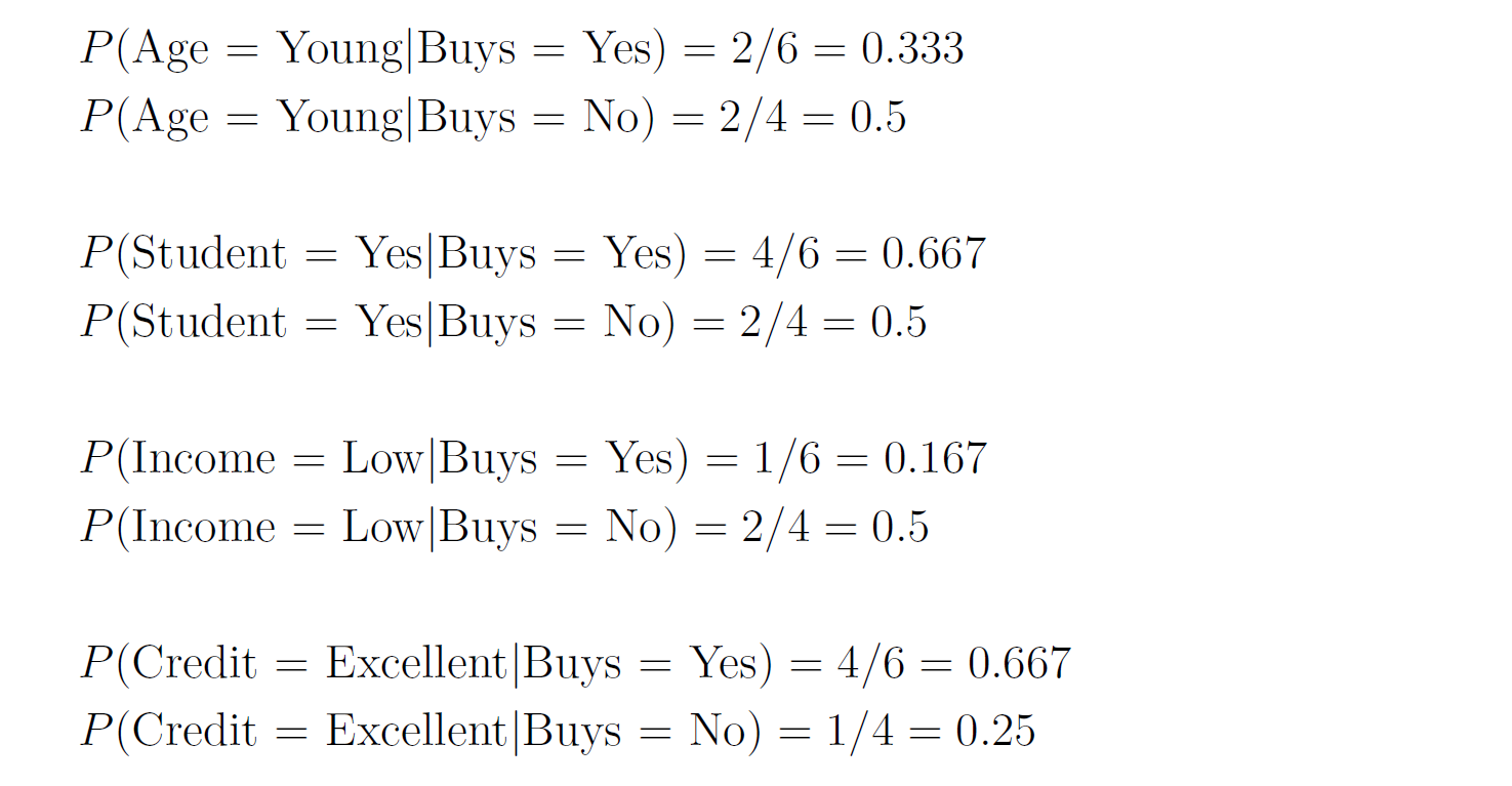 Therefore, the class posterior probabilities are: 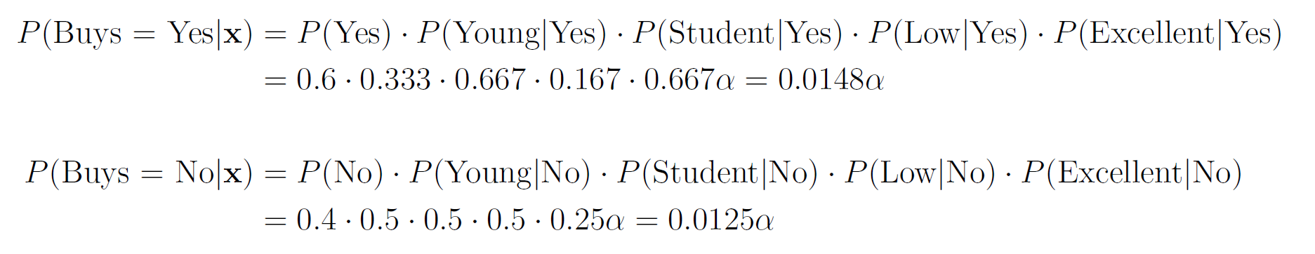 _α_ is the normalization factor (_α_ = 1 / _P_(**x**)). Since _P_(Buys = Yes|**x**) > _P_(Buys = No|**x**), our prediction is that the customer will buy the product. If we want to get the actual probability that the customer will buy the product, we can first find the normalization factor using the fact that the two posterior probabilities must sum to 1:  Then, we can plug it in the posterior probability for Buy = Yes:  The probability that the customer will buy the product is 54.21%. ## Multinomial Naive Bayes In the multinomial event model, we assume that the data set has only one categorical feature _x_ that can take one of _m_ categories, and each feature vector (_x_₁, …, _xₘ_) is a **histogram**, where _xⱼ_ counts the number of times _x_ had the value _j_ in that particular instance. This event model is particularly useful when working with text documents, where _m_ is the number of words in the vocabulary, and each feature _xⱼ_ represents the number of times the _j_th word from the vocabulary appears in the document. This representation is called the **bag-of-words** model:  In this event model, we estimate the probability _P_(_x = v_|_y_ = _k_) as the frequency in which feature _x_ gets the value _v_ in samples of class _k_:  where _nᵥₖ_ is the number of samples in class _k_ in which _x_ gets the value _v_, and _nₖ_ is the total number of samples in class _k_. ### Example: Spam Filter We would like to build a spam filter based on a training set with 100 emails: 80 of them are non-spam (ham) and 20 of them are spam. The counts of the words in each type of email are given in the following tables: 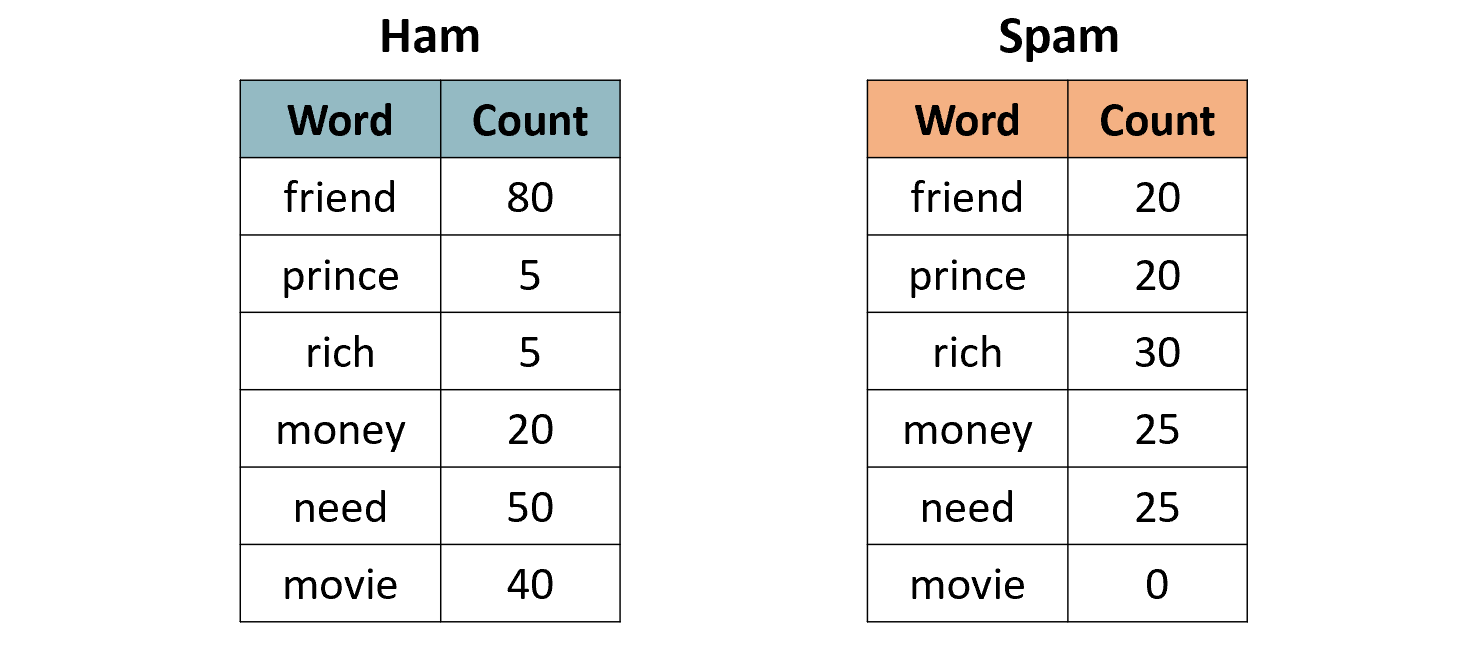 A new email has arrived with the text "rich friend need money". Is this a ham or a spam? Let's first compute the class prior probabilities: 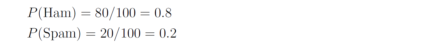 Next, we estimate the likelihoods of the words in each type of email. The total number of words in the ham emails is: 80 + 5 + 5 + 20 + 50 + 40 = 200, and the total number of words in the spam emails is: 20 + 20 + 30 + 25 + 25 = 120. Therefore, the likelihoods of the words are:  Consequently, the class posterior probabilities are: 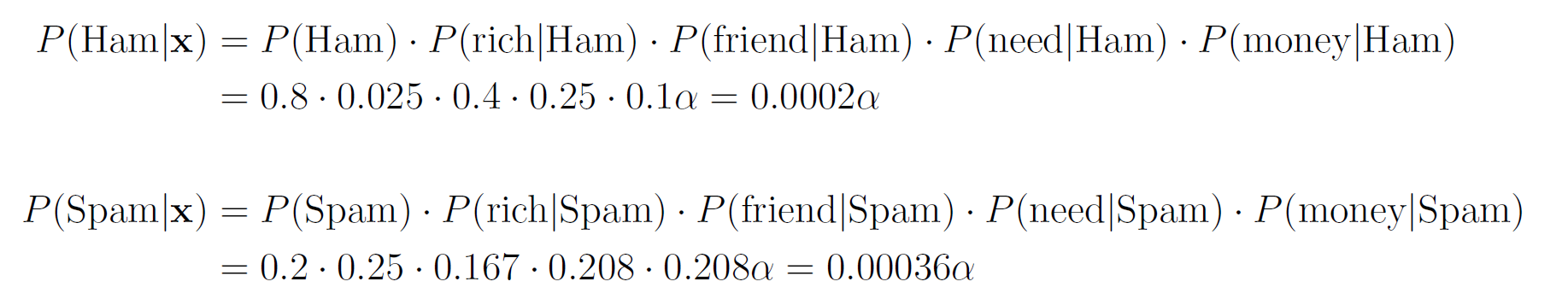 Therefore, our prediction is that the email is spam. ## Laplace Smoothing If one of the features and a given class never occur together in the training set, then the estimate of its likelihood will be zero. Since the likelihoods of the features are multiplied together, this will wipe out all the information that we have from the other features. For example, since the word "movie" is missing from the spam emails, if we get an email with the word "movie" in it, it will be automatically considered as a ham, even if the other words in the email are very "spammy". As a concrete example, consider an email with the text "movie rich rich prince". This email will be classified as a ham, although the words "rich" and "prince" are highly correlated with spam emails, because the posterior probability of Spam is zero: 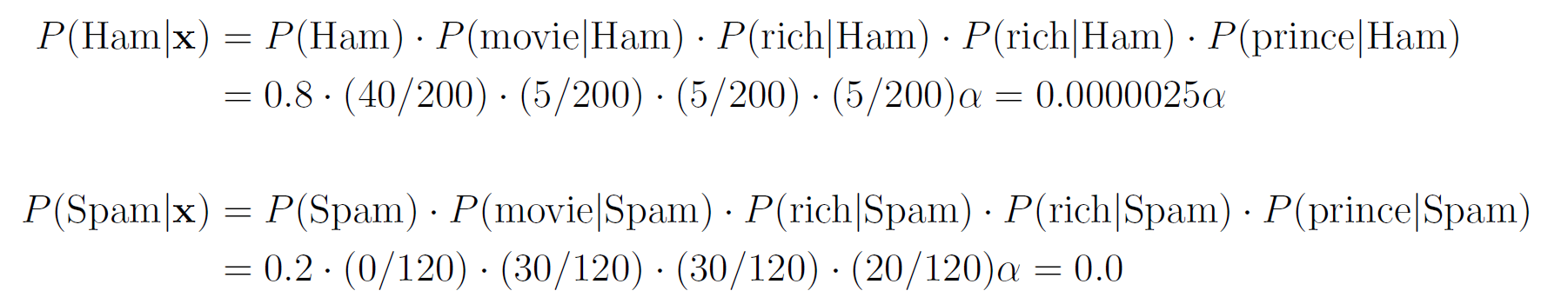 In order to deal with this issue, we incorporate a small sample correction (called pseudocount) in all the probability estimates, such that no probability is never set to exactly zero. In multinomial Naive Bayes, this correction is applied as follows:  where _α_ is a smoothing parameter and _n_ is the total number of samples in the training set. Setting _α_ = 1 is called **Laplace smoothing** (the most common one), while _α_ < 1 is called Lidstone smoothing. Similarly, in categorical Naive Bayes the correction is applied as follows:  where _nⱼ_ is the number of possible categories of feature _j_. — Revisiting our spam filter example, let's apply Laplace smoothing by adding a pseudocount of 1 to all the words:  This time, the email with the text "movie rich rich prince" will be classified as a spam, since: 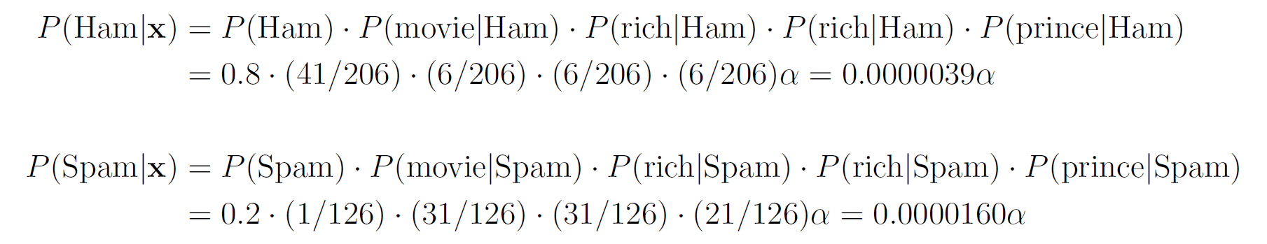 ## Gaussian Naive Bayes Up until now we assumed that all our features are discrete. How does the Naive Bayes model deal with continuous features? There are three main approaches to deal with continuous features: 1. Discretize the feature values and obtain a Bernoulli or categorically distributed features. 2. Assume that the feature is distributed according to some known probability distribution (usually a normal distribution) and estimate the parameters of that distribution from the training set (e.g., the mean and variance of the normal distribution). 3. Use [KDE (kernel density estimation)](https://en.wikipedia.org/wiki/Kernel_density_estimation) to estimate the probability density function of the feature using the given sample points as kernels. In Gaussian Naive Bayes, we take the second approach and assume that the likelihood of the features is Gaussian:  where _μⱼₖ_ is the mean of the values of _xⱼ_ in all the samples that belong to class _k_, and _σⱼₖ_ is the standard deviation of these values (these are the maximum likelihood estimates of the true parameters of the distribution). — The event models described above can also be combined in case we have a heterogenous data set, i.e., a data set that contains different types of features (for example, both categorical and continuous features). ## Naive Bayes Classifiers in Scikit-Learn The module sklearn.naive_bayes provides implementations for all the four Naive Bayes classifiers mentioned above: 1. [BernoulliNB](https://scikit-learn.org/stable/modules/generated/sklearn.naive_bayes.BernoulliNB.html#sklearn.naive_bayes.BernoulliNB) implements the Bernoulli Naive Bayes model. 2. [CategoricalNB](https://scikit-learn.org/stable/modules/generated/sklearn.naive_bayes.CategoricalNB.html#sklearn.naive_bayes.CategoricalNB) implements the categorical Naive Bayes model. 3. [MultinomialNB](https://scikit-learn.org/stable/modules/generated/sklearn.naive_bayes.MultinomialNB.html#sklearn.naive_bayes.MultinomialNB) implements the multinomial Naive Bayes model. 4. [GaussianNB](https://scikit-learn.org/stable/modules/generated/sklearn.naive_bayes.GaussianNB.html#sklearn.naive_bayes.GaussianNB) implements the Gaussian Naive Bayes model. The first three classes accept a parameter called _alpha_ that defines the smoothing parameter (by default it is set to 1.0). ## Document Classification Example In the following demonstration we will use MultinomialNB to solve a document classification task. The data set we are going to use is the [20 newsgroups dataset](https://scikit-learn.org/stable/datasets/real_world.html#newsgroups-dataset), which consists of 18,846 newsgroups posts, partitioned (nearly) evenly across 20 different topics. This data set has been widely used in research of text applications in Machine Learning, including document classification and clustering. ### Loading the Data Set You can use the function [fetch_20newsgroups()](https://scikit-learn.org/stable/modules/generated/sklearn.datasets.fetch_20newsgroups.html) in Scikit-Learn to download the text documents with their labels. You can either download all the documents as one group, or download the training set and the test set separately (using the _subset_ parameter). The split between the training and the test sets is based upon messages posted before or after a specific date. By default, the text documents contain some metadata such as headers (e.g., the date of the post), footers (signatures) and quotes to other posts. Since these features are not relevant for the text classification task, we will strip them out by using the _remove_ parameter: "`csharp from sklearn.datasets import fetch_20newsgroups train_set = fetch_20newsgroups(subset='train', remove=('headers', 'footers', 'quotes')) test_set = fetch_20newsgroups(subset='test', remove=('headers', 'footers', 'quotes')) "` Note that the first time you call this function it may take a few minutes to download all the documents, after which they will be cached locally in the folder ~/scikit_learn_data_._ The output of the function is a dictionary that contains the following attributes: – _data_ – the set of documents – _target_ – the target labels – _target_names_ – the names of the document categories Let's store the documents and their labels in proper variables: "`python X_train, y_train = train_set.data, train_set.target X_test, y_test = test_set.data, test_set.target "` ### Data Exploration Let's do some basic exploration of the data. The number of documents we have in the training and the test sets is: "`python print('Documents in training set:', len(X_train)) print('Documents in test set:', len(X_test)) "` "` Documents in training set: 11314 Documents in test set: 7532 "` A simple calculation shows that 60% of the documents belong to the training set, and 40% to the test set. Let's print the list of categories: "`python categories = train_set.target_names categories "` "` ['alt.atheism', 'comp.graphics', 'comp.os.ms-windows.misc', 'comp.sys.ibm.pc.hardware', 'comp.sys.mac.hardware', 'comp.windows.x', 'misc.forsale', 'rec.autos', 'rec.motorcycles', 'rec.sport.baseball', 'rec.sport.hockey', 'sci.crypt', 'sci.electronics', 'sci.med', 'sci.space', 'soc.religion.christian', 'talk.politics.guns', 'talk.politics.mideast', 'talk.politics.misc', 'talk.religion.misc'] "` As evident, some of the categories are closely related to each other (e.g., _comp.sys.mac.hardware_ and _comp.sys.ibm.pc.hardware_), while others are highly uncorrelated (e.g., _sci.electronics_ and _soc.religion.christian_). Finally, let's examine one of the documents in the training set (e.g., the first one): "`python print(X_train[0]) "` "` I was wondering if anyone out there could enlighten me on this car I saw the other day. It was a 2-door sports car, looked to be from the late 60s/ early 70s. It was called a Bricklin. The doors were really small. In addition, the front bumper was separate from the rest of the body. This is all I know. If anyone can tellme a model name, engine specs, years of production, where this car is made, history, or whatever info you have on this funky looking car, please e-mail. "` Unsurprisingly, the label of this document is: "`css categories[y_train[0]] "` "` 'rec.autos' "` ### Converting Text to Vectors In order to feed text documents into machine learning models, we first need to convert them into vectors of numerical values (i.e., **vectorize** the text). This process typically involves preprocessing and cleaning of the text, and then choosing a suitable numerical representation for the words in the text. **Text preprocessing** consists of various steps, amongst which the most common ones are: 1. Cleaning and normalizing the text. This includes removing punctuation marks and special characters, and converting the text into lower-case. 2. Text tokenization, i.e., splitting the text into individual words or terms. 3. Removal of stop words. Stop words are a set of commonly used words in a given language. For example, stop words in English include words like "the", "a", "is", "and". These words are usually filtered out since they do not carry useful information. 4. Stemming or lemmatization. **Stemming** reduces the word to its lexical root by removing or replacing its suffix, while **lemmatization** reduces the word to its canonical form (lemma) and also takes into account the context of the word (its part-of-speech). For example, the word _computers_ has the lemma _computer_, but its lexical root is _comput_. The following example demonstrates these steps on a given sentence: 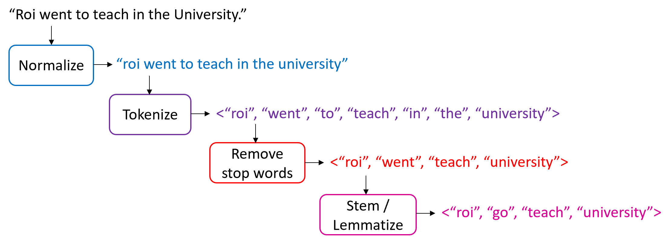 After cleaning the text, we need to choose how to vectorize it into a numerical vector. The most common approaches are: 1. **Bag-of-words (BOW) model**. In this model, each document is represented by a word counts vector (similar to the one we have used in the spam filter example). 2. **[TF-IDF](https://en.wikipedia.org/wiki/Tf%E2%80%93idf)** (Term Frequency times Inverse Document Frequency) measures how relevant a word is to a document by multiplying two metrics: (a) TF (Term Frequency) – how many times the word appears in the document. (b) IDF (Inverse Document Frequency) – the inverse of the frequency in which the word appears in documents across the entire corpus. The idea is to decrease the weight of words that occur frequently in the corpus, while increasing the weight of words that occur rarely (and thus are more indicative of the document's category). 3. **Word embeddings**. **** In this approach**,** words are mapped into real-valued vectors in such a way that words with similar meaning have close representation in the vector space. This model is typically used in deep learning and will be discussed in a future post. Scikit-Learn provides the following two transformers, which support both text preprocessing and vectorization: 1. [CountVectorizer](https://scikit-learn.org/stable/modules/generated/sklearn.feature_extraction.text.CountVectorizer.html) uses the bag-of-words model. 2. [TfIdfVectorizer](https://scikit-learn.org/stable/modules/generated/sklearn.feature_extraction.text.TfidfVectorizer.html) uses the TF-IDF representation. Important hyperparameters of these transformers include: – _lowercase_ – whether to convert all the characters to lowercase before tokenizing (defaults to True). – _token_pattern_ – the regular expression used to define what is a token (the default regex selects tokens of two or more alphanumeric characters). – _stop_words_ – if 'english', uses a built-in stop word list for English. If None (the default), no stop words will be used. You can also provide your own custom stop words list. – _max_features_ – if not None, build a vocabulary that includes only the top _max_features_ with the highest term frequency across the training corpus. Otherwise, all the features are used (this is the default). Note that these transformers do not provide advanced preprocessing techniques such as stemming or lemmatization. To apply these techniques, you will have to use other libraries such as [NLTK](https://www.nltk.org/) (Natural Language Toolkit) or [spaCy](https://spacy.io/). Since Naive Bayes models are known to work better with TF-IDF representations, we will use the TfidfVectorizer to convert the documents in the training set into TF-IDF vectors: "`python from sklearn.feature_extraction.text import TfidfVectorizer vectorizer = TfidfVectorizer(stop_words='english') X_train_vec = vectorizer.fit_transform(X_train) "` The shape of the extracted TF-IDF vectors is: "`python print(X_train_vec.shape) "` "` (11314, 101322) "` That is, there are 101,322 unique tokens in the vocabulary of the corpus. We can examine these tokens by calling the method _get_feature_names_out_() of the vectorizer: "`python vocab = vectorizer.get_feature_names_out() print(vocab[50000:50010]) # pick a subset of the tokens "` "` ['innacurate' 'innappropriate' 'innards' 'innate' 'innately' 'inneficient' 'inner' 'innermost' 'innertubes' 'innervation'] "` Evidently, there was no automatic spell checker back in the 90s

Tags: Artificial Intelligence Bayes Theorem Bayesian Machine Learning Deep Dives Machine Learning

Comment