The _travelling salesman problem (TSP)_ is a ubiquitous problem within _combinatorial optimization_ and mathematics in general. The problem poses the question: ‘Given a list of cities and their distances, what is the shortest route that visits each city once and returns to the original city?'
A more formal mathematical definition for the TSP is the Hamiltonian cycle.
The reason this problem is famous is because it is NP-hard. This essentially means you cannot find the optimal solution in a reasonable amount of time as the addition of new cities lead to a _combinatorial explosion of the number of possible routes. For example, with 4 cities the number of possible routes is 3, with 6 cities it is 60, however with 20 cities it is a huge 60,822,550,200,000,000!_
The number of solutions to the TSP is (n-1)!/2 where n is the number of cities. For large n the number of solutions is intractable by modern computing standards.
So this begs the question, how do we find the shortest distance if we have some unfathomable number of routes to try? Well, you can of course use the brute-force (naive solution) approach and try every possible route, but like we mentioned above, for a certain number of cities this can take years with current computing standards. In fact for 20 cities, it would take on the order of ~1000 years to try every route!
This is where we refer to special **[heuristic](https://en.wikipedia.org/wiki/Heuristic(computerscience))** or meta-heuristic algorithms, which don't guarantee to find the best solution every time, but will try and achieve a good-enough solution to the problem in a reasonable amount of time. In this article, we will use such an algorithm named _Simulated Annealing (SA)_ to solve the TSP.
Simulated Annealing
Overview
Simulated Annealing is a stochastic _global search algorithm which means it uses randomness as part of its search for the best solution. It derives its name and inspiration from a similar process named Annealing in Metallurgy_ whereby heating or cooling a metal affects its physical characteristics.
SA uses this concept of temperature in determining the probability of transitioning (stochasticity of the search) to a worse solution in order to more widely explore the search space and have a better chance of finding the _global optimum. This helps avoid getting stuck in a local optimum which algorithms such as Hill Climbing_ often do.
Theory
The general mathematical framework of SA is:
Equation generated by author.
Where:
Equation generated by author.
In these equations x is the current state, x' is the new state, Δy is the difference in cost or score of the two states, P(x → x') is the probability of transitioning to the new state from the current on and T is the temperature.
One can see that we always transition to the new state when it has a better score than the current one we are in. Additionally, when the temperature T is very high, we are also very likely to transition to the new site despite it having a worse score. This allows us to more easily move around and explore the search space to find the global optimum.
As the temperature decreases, we are less likely to transition to a worse solution. Therefore, the process starts to converge to an optimum and starts exploiting the search space.
The temperature is often cooled exponentially:
Equation generated by author.
Where 0 ≤ γ ≤ 1 and t is the iteration number.
Another common question is how to determine the initial temperature? This is actually quite a complex topic and I point the reader to _here_ for a research paper on the subject. In general, you can just start with a temperature that you know is high enough to accept worse solutions at the beginning. This is just a classic trial and error process!
Algorithm For TSP
The way SA can be used for the TSP is as follows:
Get an initial solution, this can be any valid route for the salesman.
Randomly select two cities and swap them in the route.
Use SA to compute the probability of whether we accept this new solution or not.
Continue this process for a set number of iterations and cool the temperature (decrease) on every iteration.
Always log the best overall solution you have found as well.
Python Implementation
Let's implement this in Python to show you a working example.
First we will generate some data points, which will be our cities:
Plot generated by author in Python.
The plot above is our cities along with an initial solution. The initial solution was simply generated by going through the cities in alphabetical order e.g. a, b, c … r, s, a. We have 20 cities, which means we have a breathtaking total of 60,822,550,200,000,000 different possible routes to try!
Now we will build a Python class to carry out the Simulated Annealing process for the TSP!
I am not the best coder in Python, so I appreciate the following snippet may not be the best implementation …
We will now run the SA Optimization algorithm and plot the solution:
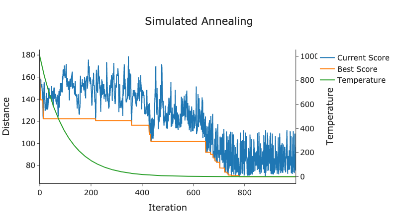
Plot generated by author in Python.
Plot generated by author in Python.
The above plots show the solutions we iterated over plotted alongside the temperature and the best current solution. The bottom plot shows the route of the best solution we found through the SA algorithm. From a simple ‘eye-test' this new solution is much better than the initial and seems to be quite optimal.
Summary
In this post we have gone over the travelling salesman problem, which asks us to find the shortest route for a set of cities (points). The number of possible different routes explodes as we add more cities and cannot be solved brute-force. However, we can make use of a meta-heuristic algorithm such as Simulated Annealing (SA) to find sufficient solution in most cases.
The full code used in the article can be found at my GitHub here:
I have a free newsletter, Dishing the Data, where I share weekly tips for becoming a better Data Scientist. There is no "fluff" or "clickbait," just pure actionable insights from a practicing Data Scientist.