Courage to Learn ML: A Detailed Exploration of Gradient Descent and Popular Optimizers

Welcome back to a new chapter of ‘Courage to Learn ML. For those new to this series, this series aims to make these complex topics accessible and engaging, much like a casual conversation between a mentor and a learner, inspired by the writing style of "The Courage to Be Disliked," with a specific focus on machine learning.
In our previous discussions, our mentor and learner discussed about some common loss functions and the three fundamental principles of designing loss functions. Today, they'll explore another key concept: gradient descent.
As always, here's a list of the topics we'll be exploring today:
- What exactly is a gradient, and why is the technique called ‘gradient descent'?
- Why doesn't vanilla gradient descent perform well in Deep Neural Networks (DNNs), and what are the improvements?
- A review of various optimizers and their relationships (Newton's method, Adagrad, Momentum, RMSprop, and Adam)
- Practical insights on selecting the right optimizer based on my personal experience
So, we've set up the loss function to measure how different our predictions are from actual results. To close this gap, we adjust the model's parameters. Why do most algorithms use gradient descent for their learning and updating process?
To address this question, let's imagine developing a unique update theory, assuming we're unfamiliar with gradient descent. We start by using a loss function to quantify the discrepancy, which encompasses both the signal (the divergence of the current model from the underlying pattern) and noise (such as data irregularities). The subsequent step involves conveying this data and utilizing it to adjust various parameters. The challenge then becomes determining the extent of modification needed for each parameter. A basic approach might involve calculating the contribution of each parameter and updating it proportionally. For instance, in a linear model like W*x + b = y, if the prediction is 50 for x = 1 but the actual value is 100, the gap is 50. We could then compute the contribution of w and b, adjusting them to align the prediction with the actual value of 100.
However, two significant issues arise:
- Calculating the Contribution: With many potential combinations of w and b that could yield 100 when x = 1, how do we decide which combination is better?
- Computational Demand in Complex Models: Updating a Deep Neural Network (DNN) with millions of parameters could be computationally demanding. How can we efficiently manage this?
These difficulties highlight the complexity of the problem. It's nearly impossible to accurately determine each parameter's contribution to the final prediction, especially in non-linear and intricate models. Therefore, to update model parameters effectively based on the loss, we need a method that can precisely dictate the adjustments for each parameter without being computationally costly.
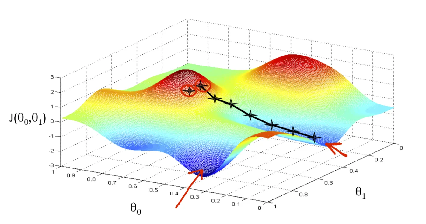
Thus, rather than focusing on how to allocate loss across each parameter, we could consider it as a strategy to traverse the loss surface. The objective is to locate a set of parameters that guide us to the global minimum – the closest approximation achievable by the model. This adjustment process is akin to playing an RPG game, where the player seeks the lowest point in a map. This is the foundational idea behind gradient descent.

So what is exactly gradient descent? Why it call gradient descent?
Let's break it down. The loss surface, central to optimization, is shaped by the loss function and model parameters, varying with different parameter combinations. Imagine a 3D loss surface plot: the vertical axis represents the loss function value, and the other two axes are the parameters. At the global minimum, we find the parameter set with the lowest loss, our ultimate target to minimize the gap between actual results and our predictions.

But how do we navigate towards this global minimum? That's where the gradient comes in. It guides us in the direction to move. You might wonder, why calculate the gradient? Ideally, we'd see the entire loss surface and head straight for the minimum. But in reality, especially with complex models and numerous parameters, we can't visualize the entire landscape – it's more complex than a simple valley. We can only see what's immediately around us, like being in a foggy landscape in an RPG game. So, we use the gradient, which points towards the steepest ascent, and then head in the opposite direction, towards the steepest descent. By following the gradient, we gradually descend to the global minimum on the loss surface. This journey is what we call gradient descent.

How exactly does gradient descent decide the adjustments needed for each parameter, and why is it more effective than our initially proposed simple method?
Our objective is to minimize the loss function with a particular set of parameters, achievable only by adjusting these parameters. We indirectly influence the loss function through these changes.
Let's revisit our RPG analogy. The hero, with only basic movements (left/right, forward/backward) and limited visibility, aims to find the lowest point on an uncharted map to unearth a legendary weapon. We know the gradient indicates the direction to move, but it's more than just a pointer. It also decomposes into fundamental movements.
The gradient, a vector of partial derivatives with respect to each parameter, signifies how much and in which basic direction (left, right, forward, backward) to move. It's like a magical guide not only pointing to the hill's left side will lead us to the legendary weapon but also instructing specific turns and steps to take.
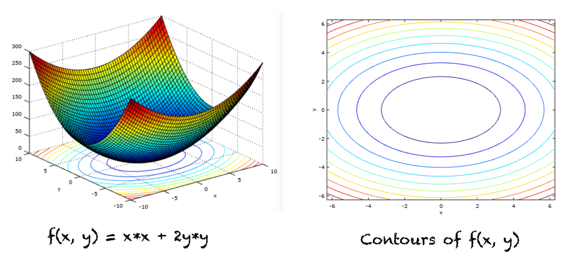
However, it's crucial to understand what the gradient actually is. Often tutorials suggest imagining you're on a hill and looking around to choose the steepest direction to descend. But this can be misleading. The gradient isn't a direction on the loss surface itself but a projection of that direction onto the parameter dimensions (in the graph, the x,y coordinates), guiding us in the loss function's minimal direction. This distinction is crucial – the gradient isn't on the loss surface but a directional guide within the parameter space.

That's why most visualizations use parameter contours, not the loss function to illustrate gradient descent processes. The movement is about adjusting parameters, with changes on the loss function being a consequence.

Gradient is formed by partial derivatives. A partial derivative, on the other hand, helps us understand how a function changes in relation to a specific parameter, holding others constant. This is how gradients quantify each parameter's influence on the loss function's directional change.
Gradient descent naturally and efficiently resolves the parameter tuning dilemma we initially faced. It's especially adept at locating global minima in convex problems and local minima in nonconvex scenarios. Modern implementations benefit from parallelization and acceleration via GPUs or TPUs. Variations like mini-batch gradient descent and Adam optimize its efficiency across different contexts. In summary, gradient descent is stable, capable of handling large datasets and numerous parameters, making it a superior choice for our learning purposes.
